Robotics toolbox examples

Installing robotics toolbox

Robotics toolbox can be easily downloaded as sa pip package or our preferred way using anaconda.

Pip package install

Install the robotics toolbox

pip install roboticstoolbox-python

If you still have not installed pycapacity, you can install it using

pip install pycapacity

Then if you want to use Swift, install the package for dealing with meshes called trimesh

pip install trimesh

Finally the package called networkx for displaying the robot in Swift correctly

pip install networkx

Anaconda install

For anaconda instals you can simply download the yaml file and save it as env.yaml:

name: rtbx_examples
channels:
  - conda-forge
dependencies:
  - python=3.8
  - roboticstoolbox-python
  - numpy
  - matplotlib
  - pip
  - pip:
    - pycapacity
    - trimesh

And create a new ready to go environment:

conda env create -f env.yaml    # create the new environemnt and install robotics toolbosx, pycapacity, ...
conda activate rtbx_examples

Creating the custom environment from scratch

You can also simply use anaconda to create a new custom environment:

conda create -n rtbx_examples python=3.8 # create python 3.8 based environment
conda activate rtbx_examples
conda install -c conda-forge roboticstoolbox-python numpy matplotlib 

Then install pycapacity for the workspace analysis

pip install pycapacity

📢 NEW Examples!

For some more examples check out the examples folder of the repository.

• Interactive jupyter notebooks are available in the examples/notebooks folder: see on Github

• Python scripts are available in the examples/scripts folder: see on Github

Code example using pyplot

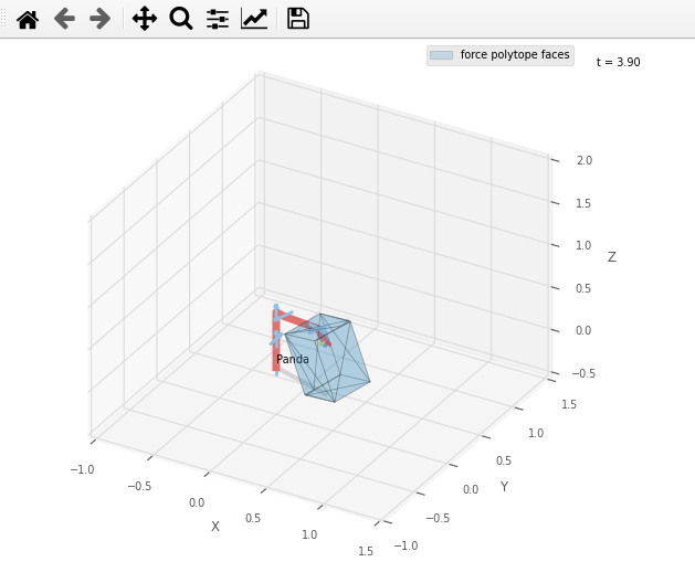
Calculating the force polytope of the panda robot and visualising it using the pyplot.

import roboticstoolbox as rp
import numpy as np

panda = rp.models.DH.Panda()
# initial pose
q= np.array([0.00138894 ,5.98736e-05,-0.30259058,   -1.6, -6.64181e-05,    1.56995,-5.1812e-05])
panda.q = q
# joint torque limits
t_max = np.array([87, 87, 87, 87, 20, 20, 20]) 
t_min = -t_max

# polytope python module
import pycapacity.robot as pyc

# robot matrices
Jac = panda.jacob0(q)[:3,:]
# gravity torque
gravity = panda.gravload(q).reshape((-1,1))

# calculate for the polytope
f_poly =  pyc.force_polytope(Jac, t_max, t_min, gravity)

# plotting the polytope using pycapacity
import matplotlib.pyplot as plt
from pycapacity.visual import * # pycapacity visualisation tools

# visualise panda
fig = panda.plot(q)
ax = fig.ax

# draw faces and vertices
plot_polytope(plot=plt, 
              polytope=f_poly, 
              label='force polytope',
              edge_color='black', 
              alpha = 0.2, 
              show_vertices=False,
              center=panda.fkine(q).t,  # set the polytope center at the end effector position
              scale=1/500) # scale the polytope and place it to the end-effector

ax.set_xlim([-1, 1.5])
ax.set_ylim([-1, 1.5])
ax.set_zlim([0, 1.5])
plt.legend()
plt.show()
fig.hold()

📢 NEW Examples!

For some more examples check out the examples folder of the repository.

• Interactive jupyter notebooks are available in the examples/notebooks folder: see on Github

• Python scripts are available in the examples/scripts folder: see on Github

Code example using Swift

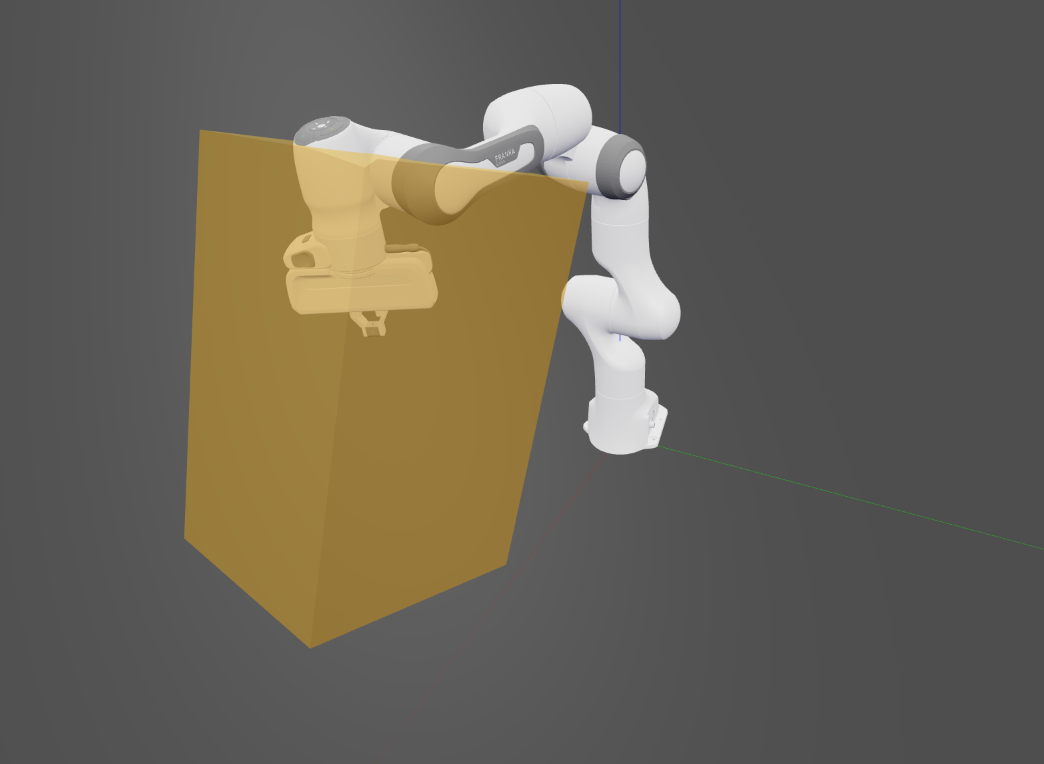
Calculating the force polytope of the panda robot and visualising it using the Swift.

import roboticstoolbox as rp
import numpy as np

panda = rp.models.DH.Panda()
# initial pose
q= np.array([0.00138894 ,5.98736e-05,-0.30259058,   -1.6, -6.64181e-05,    1.56995,-5.1812e-05])
panda.q = q
# joint torque limits
t_max = np.array([87, 87, 87, 87, 20, 20, 20]) 
t_min = -t_max

# polytope python module
import pycapacity.robot as pyc

# robot matrices
Jac = panda.jacob0(q)[:3,:]
# gravity torque
gravity = panda.gravload(q).reshape((-1,1))

# calculate for the polytope
f_poly =  pyc.force_polytope(Jac, t_max, t_min, gravity)
# calculate the face representation of the polytope
f_poly.find_faces()

 # visualise panda
panda = rp.models.Panda()
import swift.Swift as Swift
panda.q = q
env = Swift()
env.launch()
env.add(panda)


# polytope visualisation
import trimesh
# save polytope as mesh file
scaling = 500
# create the mesh
mesh = trimesh.Trimesh(vertices=(f_poly.vertices.T/scaling + panda.fkine(q).t),
                       faces=f_poly.face_indices, use_embree=True, validate=True)

# absolute path to the temporary polytope file saved 
# in the stl format
import os
file_path = os.path.join(os.getcwd(),'tmp_polytope_file.stl')
                  
f = open(file_path, "wb")
f.write(trimesh.exchange.stl.export_stl(mesh))
f.close()
# robot visualisation
from spatialgeometry import Mesh
poly_mesh = Mesh(file_path)
poly_mesh.color = (0.9,0.6,0.0,0.5)
env.add(poly_mesh)

📢 NEW Examples!

For some more examples check out the examples folder of the repository.

• Interactive jupyter notebooks are available in the examples/notebooks folder: see on Github

• Python scripts are available in the examples/scripts folder: see on Github

Code example using matplotlib

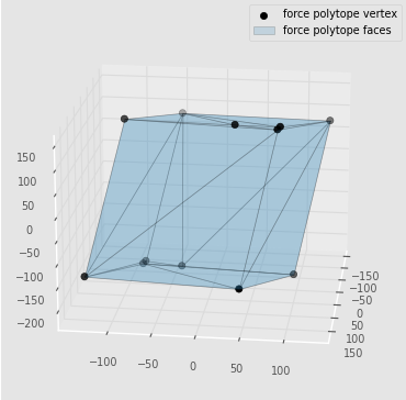
Calculating the force polytope of the panda robot only polytope using matplotlib

import roboticstoolbox as rp
import numpy as np

panda = rp.models.DH.Panda()
# initial pose
q= np.array([0.00138894 ,5.98736e-05,-0.30259058,   -1.6, -6.64181e-05,    1.56995,-5.1812e-05])
panda.q = q
# joint torque limits
t_max = np.array([87, 87, 87, 87, 20, 20, 20]) 
t_min = -t_max

# polytope python module
import pycapacity.robot as pyc

# robot matrices
Jac = panda.jacob0(q)[:3,:]
# gravity torque
gravity = panda.gravload(q).reshape((-1,1))

# calculate for the polytope
f_poly = pyc.force_polytope(Jac, t_max, t_min, gravity)

# plotting the polytope using pycapacity
import matplotlib.pyplot as plt
from pycapacity.visual import * # pycapacity visualisation tools
fig = plt.figure()

# draw polytope
plot_polytope(plot=plt, 
              polytope=f_poly, 
              label='force polytope',
              edge_color='black', 
              alpha = 0.2,)

plt.legend()
plt.show()