Reachable Space with Pinocchio and CGAL

This is an example tutorial of how to setup pinocchio and CGAL library with pycapacity to calculate and visualise the robot capacities

../_images/reachable.gif

Installing Pinocchio

Pinocchio library can be downloaded as sa pip package however due to the large number of different dependencies we suggest you to use anaconda.

Pip package install

Install the pinocchio library

pip install pin

Install an additional library with robot data example_robot_data provided by pinocchio community as well more info

pip install example-robot-data

Install the visualisation library meshcat that is compatible with pinocchio simple and powerful visualisaiton library more info

pip install meshcat

Then install CGAL library for the workspace analysis

pip install cgal

Finally install pycapacity for the workspace analysis

pip install pycapacity

Also you can install ipython of jupyter for simplicity.

Anaconda install

For anaconda instals you can simply download the yaml file and save it as env.yaml:

name: rwspace
channels:
  - defaults
  - conda-forge
dependencies:
  - python
  - conda-forge::pinocchio
  - conda-forge::gepetto-viewer
  - conda-forge::gepetto-viewer-corba
  - conda-forge::example-robot-data
  - conda-forge::meshcat-python
  - pip:
    - pycapacity
    - cgal

And create a new ready to go environment:

conda env create -f env.yaml    # create the new environemnt and install pinocchio, gepetto, pycapacity,.. 
conda actvavte rwspace

Creating the custom environment from scratch

You can also simply use anaconda to create a new custom environment:

conda create -n rwspace python=3 pip # create python 3.8 based environment
conda activate rwspace

Install all the needed packages

conda install -c conda-forge pinocchio 
conda install -c conda-forge example-robot-data 
conda install -c conda-forge gepetto-viewer

Then install CGAL library for the workspace analysis

pip install cgal

Then install pycapacity for the workspace analysis

pip install pycapacity

Code example

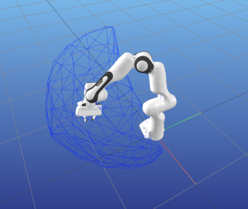
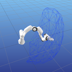
This example code calculates the reachable space of the panda robot (in a random joint configuration) and visualises it using meshcat.

import pinocchio as pin
import numpy as np
import time
from example_robot_data import load

robot = load('panda')

# Display a robot configuration.
# q0 = pin.neutral(robot.model)
q0 = robot.q0

# calculate the jacobian
data = robot.model.createData()
pin.framesForwardKinematics(robot.model,data,q0)

# set the time-horizon
horizon_time = 0.2 # secs

# create a simple forward kinematics function
# taking the current joint configuration q
# and outputting the end-effector position
def fk(q):
    pin.framesForwardKinematics(robot.model,data,q)
    return data.oMf[robot.model.getFrameId(robot.model.frames[-1].name)].translation

# polytope python module
import pycapacity.robot as pycap
# get max torque
q_max = robot.model.upperPositionLimit.T
q_min = robot.model.lowerPositionLimit.T
# get max velocity
dq_max = robot.model.velocityLimit
dq_min = -dq_max

# set a random joint configuration
q = np.random.uniform(q_min,q_max)

opt = {
  'calculate_faces': True,
  'convex_hull': False, # if True, the reachable space will be approximated with a convex hull of the vertices (does not require CGAL)
  'n_samples':3,     # number of samples per dimension of the facet (the higher the better the approximation - n_samples^facet_dim samples)
  'facet_dim':2        # dimension of the joint-space facet to be sampled (0 for vertices, 1 for edges, 2 for faces, up to n_dof -1, where n_dof is the number of degrees of freedom)
}

# calculate force polytope
rw_poly = pycap.reachable_space_nonlinear(
            forward_func=fk,
            q0=q,
            q_max= q_max, 
            q_min= q_min,
            dq_max= dq_max,
            dq_min= dq_min,
            time_horizon=horizon_time,
            options=opt
    )


## visualise the robot
from pinocchio.visualize import MeshcatVisualizer

viz = MeshcatVisualizer(robot.model, robot.collision_model, robot.visual_model)
# Start a new MeshCat server and client.
viz.initViewer(open=True)
# Load the robot in the viewer.
viz.loadViewerModel()
viz.display(q)
# small time window for loading the model 
# if meshcat does not visualise the robot properly, augment the time
# it can be removed in most cases
time.sleep(0.2) 

## visualise the polytope and the ellipsoid
import meshcat.geometry as g 

# meshcat triangulated mesh
poly = g.TriangularMeshGeometry(vertices=rw_poly.vertices.T, faces=rw_poly.face_indices)
viz.viewer['rwspace'].set_object(poly, g.MeshBasicMaterial(color=0x0022ff, wireframe=True, linewidth=3, opacity=0.2))

Here is the visualisation of the reachable space of two different runns of the code:

../_images/reachable_space.png ../_images/reachable_space2.png

Animate polytopes in Meshcat

This example code calculates the reachable space of the panda robot for a sinusoidal motion and visualises it using meshcat.

import pinocchio as pin
import numpy as np

from example_robot_data import load

# get panda robot usinf example_robot_data
robot = load('panda')

# get joint position ranges
q_max = robot.model.upperPositionLimit.T
q_min = robot.model.lowerPositionLimit.T
# get max velocity
dq_max = robot.model.velocityLimit
dq_min = -dq_max

# Use robot configuration.
q = (q_min+q_max)/2

## visualise the robot
from pinocchio.visualize import MeshcatVisualizer

viz = MeshcatVisualizer(robot.model, robot.collision_model, robot.visual_model)
# Start a new MeshCat server and client.
viz.initViewer(open=True)
# Load the robot in the viewer.
viz.loadViewerModel()
viz.display(q)


import pycapacity.robot as pycap
import meshcat.geometry as g 

# set the time-horizon
horizon_time = 0.2 # secs

# create a simple forward kinematics function
# taking the current joint configuration q
# and outputting the end-effector position
def fk(q):
    pin.framesForwardKinematics(robot.model,data,q)
    return data.oMf[robot.model.getFrameId(robot.model.frames[-1].name)].translation

  opt = {
    'calculate_faces': True,
    'convex_hull': False, # if True, the reachable space will be approximated with a convex hull of the vertices (does not require CGAL)
    'n_samples':2,     # number of samples per dimension of the facet (the higher the better the approximation - n_samples^facet_dim samples)
    'facet_dim':1        # dimension of the joint-space facet to be sampled (0 for vertices, 1 for edges, 2 for faces, up to n_dof -1, where n_dof is the number of degrees of freedom)
  }

while True:
    # some sinusoidal motion
    for i in np.sin(np.linspace(-np.pi,np.pi,200)):

        # update the joint position
        q[0] = i
        q[1] = i
        q[2] = i

        # calculate the jacobian
        data = robot.model.createData()
        
        # calculate force polytope
        rw_poly = pycap.reachable_space_nonlinear(
                    forward_func=fk,
                    q0=q,
                    q_max= q_max, 
                    q_min= q_min,
                    dq_max= dq_max,
                    dq_min= dq_min,
                    time_horizon=horizon_time,
                    options=opt
            )

        # visualise the robot
        viz.display(q)

        
        # meshcat triangulated mesh
        poly = g.TriangularMeshGeometry(vertices=rw_poly.vertices.T, faces=rw_poly.face_indices)
        viz.viewer['rwspace'].set_object(poly, g.MeshBasicMaterial(color=0x0022ff, wireframe=True, linewidth=3, opacity=0.2))

../_images/rwspace_animation.gif

📢 NEW Examples!

For some more examples check out the examples folder of the repository.

Interactive jupyter notebooks are available in the examples/notebooks folder: see on Github velocity polytope and reachable space polytope
Python scripts are available in the examples/scripts folder: see on Github